In software engineering, scalability is the idea that a system should be able to handle an increase in workload by employing more computing resources without significant changes to its design.

Why don’t systems scale

Software, though “virtual”, needs physical machines to run. And physical machines are bound by the law of physics. The speed of light limits how fast a CPU can read data from memory. The information-carrying capacity of wires determines how much data can be moved from one part of a system to another. Material sciences dictate how fast a hard disk can spin to let data be read/written.

Collectively, all this means that there are hard limits to how fast our programs can run or how much work they can do. We can be very efficient within these limits, but we cannot breach them. Therefore, we are forced to use software or hardware design tricks to get our programs to do more work.

The problem of scalability is one of designing a system that can bypass the physical limits of our current hardware to serve greater workloads. Systems don’t scale because either they use the given hardware poorly, or because they cannot use all the hardware available to them e.g. programs written for CPUs won’t run on GPUs.

To build a scalable system, we must analyze how the software plays with hardware. Scalability lives at the intersection of the real and the virtual.

The key axes of scalability

Latency

This is the time taken to fulfil a single request of the workload. The lower the latency, the higher the net output of the system can be since we can process many more requests per unit time by finishing each one fast. Improving latency can be understood in terms of “speed up” (processing each unit of workload faster) and is typically achieved by splitting up the workload into multiple parts which execute in parallel.

Throughput

The other axis of scalability is how much work can be done per unit time. If our system can serve only one request at a time, then throughput = latency X time. But most modern CPUs are multicore. What if we use all of them at once? In this way (and others), we can increase the total of “concurrent” requests a system can handle. Along with latency, this defines the total things happening in a system at any point in time. This can be thought of in terms of “scale up” or concurrency.

Little’s law gives a powerful formulation of this which lets us analyze how a system and its subsystems will function under increasing load.

If the number of items in the system’s work queue keeps growing, it will eventually be overwhelmed.

Capacity

This is the theoretical maximum amount of work the system can handle. Any more load and the system starts to fail either completely or for individual requests.

Performance is not Scalability

A system with high performance is not necessarily a scalable system. Ignoring scalability concerns can often result in a much simpler system which is very efficient for a given scale but will fail completely if the workload increases.

An example of a performant yet non-scalable system is a file parser that can run on a single server and process a file up to a few GBs in a few minutes. This system is simple and serves well enough for files that will fit in the memory of one machine. A scalable version of this may be a Spark job that can read many TBs of data stored across many servers and process it using many compute nodes.

If we know that the workload is going to increase, we should go for a scalable design up-front. But if we are not sure of what the future looks like, a performant but non-scalable solution is a good enough starting point.

Quantifying scalability

Amdahl’s Law

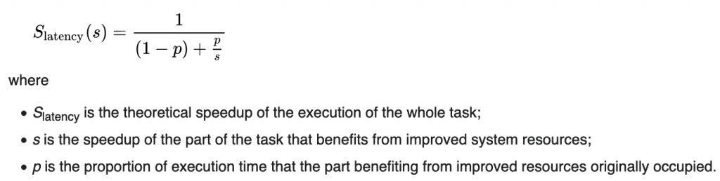
Other than the problems with implementations, there are theoretical limitations to how much faster a program can become with the addition of more resources. Amdahl’s law (presented by Gene Amdahl in 1967) is a key law that defines them.

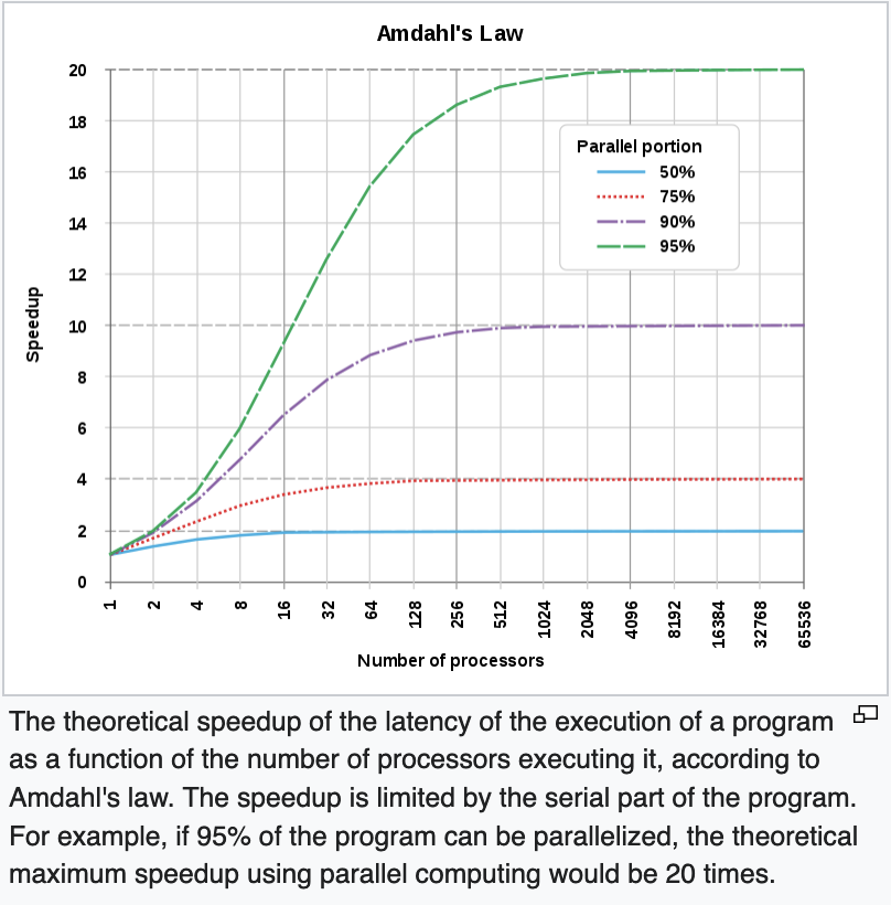
It states that every program contains part(s) that can be made to execute in parallel given extra resources, and part(s) that can only run serially (called serial fraction). As a result, there is a limit on how much faster a program can become regardless of how many resources are available to it. The total speedup is the sum of time taken to run the serial part plus the time taken to run the parallel part. The serial part, therefore, creates an upper bound on how fast a program can run with more resources.

This means that by analyzing our program structure, we can determine the maximum amount of resources that it makes sense to dedicate to speed it up – any more would be useless.

Universal Scalability Law (USL)

While Amdahl’s law defines the maximum amount of extra resources which will improve a program’s performance by allowing parts of the program to run in parallel, it ignores a key overhead in adding more resources – the communication overhead in distributing and managing work among all the new processors/machines.

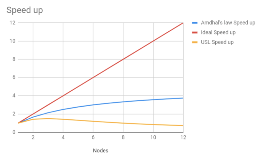
USL formalizes this by adding another factor to Ahmdahl’s Law which incorporates the cost of communication. This further reduces the net gain we can get from the addition of resources and provides a more realistic measure of how much a program can be sped up.

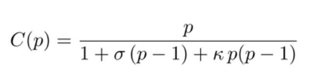
Real-world tests show that in the worst case, these communication overheads build up exponentially as each new resource is added. Program performance improves in the beginning due to more resources, but this improvement is eventually overwhelmed by the communication overhead.

Strategies for scaling systems

Vertical scalability

Vertical scalability says that if our computer is not powerful enough to run a program, we simply procure a computer that is. This is the simplest approach because we don’t have to make any change to the system itself, just the hardware it runs on. Supercomputers are a manifestation of this strategy of scalability.

This is essentially throwing money at the problem to avoid design complexity. We can build more powerful computers, but the cost of doing so gets exponentially larger. And there are limits to even that. We certainly can’t build a computer powerful enough to run the entirety of Google.

So the vertical scalability strategy can take us a good way, but it is not enough in the face of most modern scale requirements. To scale further, we need to make fundamental changes to our program itself.

Horizontal scalability

The simplest computer program is one that runs on one computer. The limits of vertical scalability indicate that the fundamental bottleneck in serving web-scale workloads is that our programs are bound to one computer.

Horizontal scalability is the process of designing systems that can utilize multiple computers to achieve a single task. If this can be achieved, then scaling the system is a simple matter of adding more and more computers instead of being forced to build a single extra-large computer.

The challenges of “distributing” a program can be far harder than the actual logic of the program itself. We must now deal not just with computers, but with the wires between those computers. The fallacies of distributed computing are very real, and demand that horizontal scalability be baked into the very fabric of the program instead of being tacked on from above.

Distributed systems

In embracing horizontal scalability, we embrace distributed systems – systems in which various computing resources like CPU, storage, and memory are located across multiple physical machines. These are complicated architectures, so let’s go through some main approaches.

Distributing data

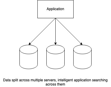
Stored data typically represents the state of the system as it would be if there were no active processing going on. To store web-scale data, we have no choice but to split its storage across many machines. While this means that we have no storage limitation, the problem now is how to locate on which server is the specific data point located. e.g. If I store millions of songs across hundreds of hard disks, how do I find one particular song?

Various techniques are used to solve this problem. Some of them are based on selecting which server to use in a smart, predetermined way so that the same logic can be applied while reading the data. These are simple techniques but somewhat brittle because the apriori logic needs to be updated constantly as the number of storage servers increases or decreases. Shard id or modulo based implementations are an example of this approach.

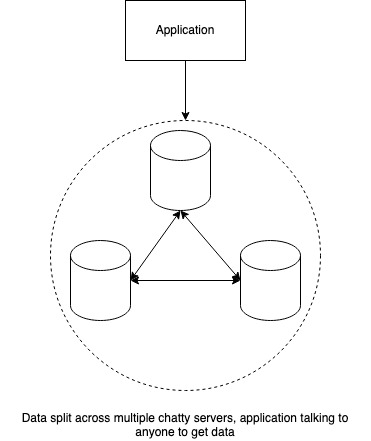
Some other techniques are based on building a shared index to locate data across the set of servers. Servers talk to each other to find and return the data required while the actual reading program is unaware of how many servers there are. Cassandra’s peer to peer approach is an example of this.

Distributing Compute

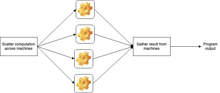
A computation or the running of a program typically modified the data owned by the system and therefore changes its state. Being able to leverage the CPU cores of multiple machines means that we have far more computing power to run our programs than with just one machine.

But if all our CPUs are not located in one place, then we need a mechanism to distribute work among them. Such a mechanism, by definition, is not part of the “business logic” of the program, but we may be forced to modify how the business logic is implemented so that we can split it into parts and run it on different CPUs.

Two situations are possible here – the CPUs may simultaneously work on the same piece of data (shared memory), or they may be completely independent (shared-nothing).

In the former, we not only have to distribute the compute to multiple servers but also have to control how these multiple servers access and modify the same pieces of data. Similar to multi-threaded programming on a single server, such architecture imposes expensive coordination constraints via distributed locking and transaction management techniques (e.g. Paxos).

The shared-nothing architecture is far more scalable because any given piece of data is only being processed in one place at a point in time and there is no danger of overlapping or conflicting changes. The problem becomes one of ensuring that such data localization happens and in finding where this piece of compute is running.

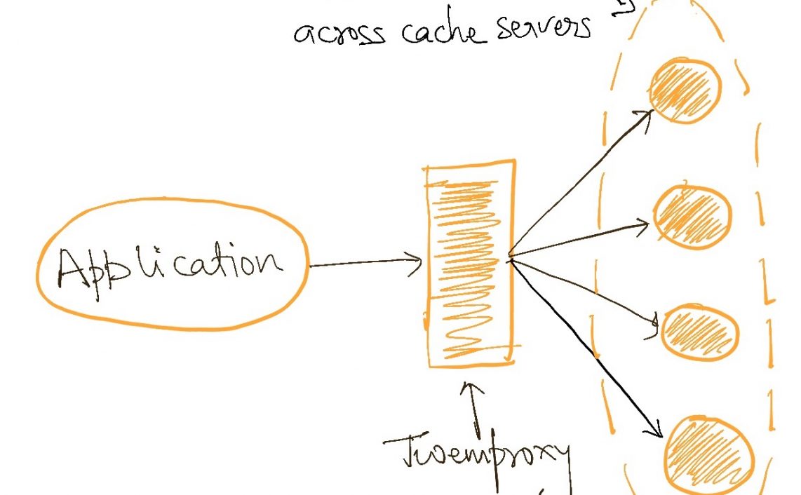
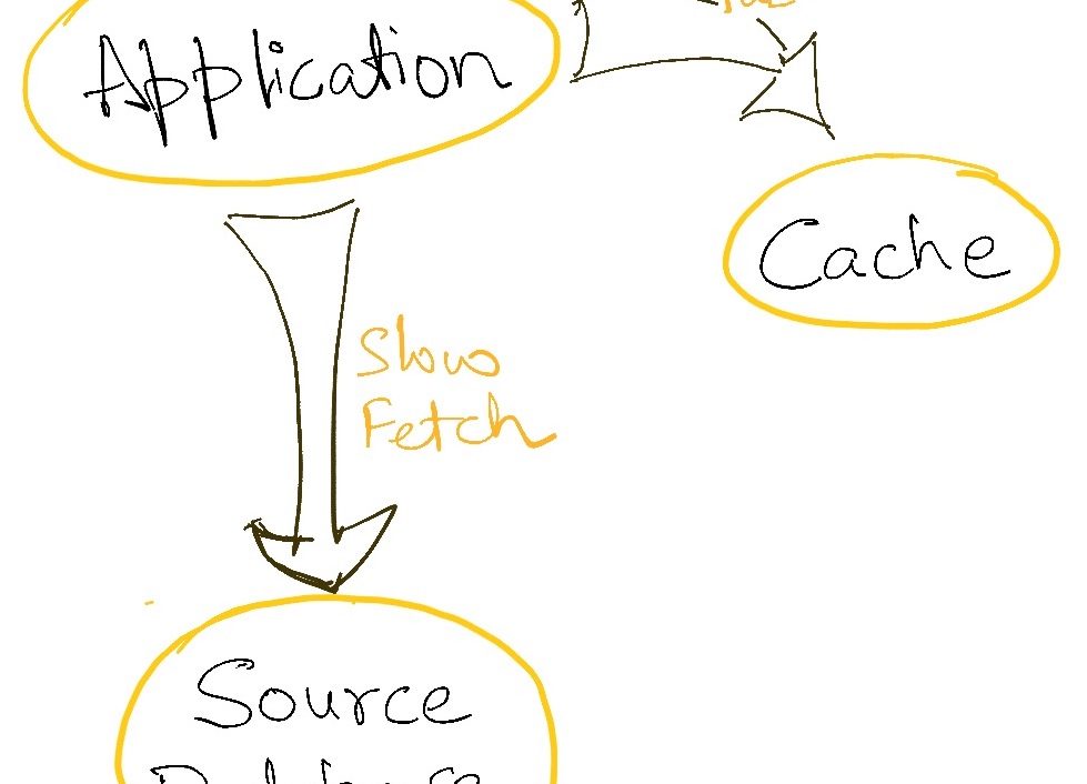
Replicating data

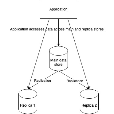
This is a hybrid scenario where even though our data fit on one or more machines, we deliberately replicate it across multiple machines simply because the current servers are not able to bear the compute load of reading and writing this data. Essentially there is so much processing going on that to be able to distribute compute, we are forced to distribute data as well (or at least copies of it).

Using read replicas of databases to scale read-heavy systems, or using caches are an example of this strategy.

Considerations in distributed computing

When we build a distributed system, we should be clear about what we expect to achieve. We should also be clear about what we will NOT get. Let’s consider both of these things while assuming that we are designing the system well.

What we won’t get

Consistency

Eric Brewer defined the CAP theorem which says that in the face of a network partition (the network breaking down and making some machines of the system inaccessible), a system can choose to maintain either availability (continuing to function) or consistency (maintaining information parity across all parts of the system). This can be intuitively understood by considering that if some machines are inaccessible, either the other should stop working (become unavailable) because they cannot modify data on the inaccessible servers, or continue to function at the risk of not updating the data on the missing machines (becoming inconsistent).

Most modern systems choose to be inconsistent rather than fail altogether so that at least parts of the systems can function. The inconsistency is later reconciled by using techniques like CRDTs.

Simplicity

A distributed system design is inevitably more complex at all levels from the networking layer upwards than a single-server architecture. So we should expect complexity and try to tackle it with good design and evolved tools.

Reduction in errors

A direct side effect of a more complicated architecture is an increase in the number of errors. Having more servers, more inter-server connections, and just more load on this scalable system is bound to result in more system errors. This can look (sometimes correctly) like system instability, but a good design should ensure that these errors are fewer per unit workload and that they remain isolated.

What we must get

Scalability

This is obvious in the context of this article. We are building distributed systems to achieve scalability, so we must get this.

Failure Isolation

This is not an outcome but an important guardrail in designing a distributed system. If we fail to isolate the increasing number of errors, the system will be brittle with large parts failing at once. Ideal distributed system design isolates errors in specific workflows so that other parts can function properly.

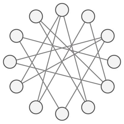
Why are distributed systems hard?

In a word – coupling.

While there are many types of coupling in software engineering, there are two which play a major role in hindering system scalability.

Both of them derive from a single server program’s assumption of “global, consistent system state” which can be modified “reliably”. Consistent state means that all parts of a program seem the same data. Reliable modification of the system’s state means that all parts of the system are always available and can be reached/invoked to modify it. But as we have seen, the CAP theorem explicitly outlaws the consistency-availability-invocability in a distributed system. This makes the leap from single server architecture to distributed architecture very difficult.

Let’s look at both these types of coupling.

Location Coupling

Location coupling is when a program assumes that something is available at a known, fixed location. e.g. A file parsing program assumes that the file is located on its local file system. or a service assuming its database is available at a given fixed location. or a subpart of a system assuming that another subpart is part of the same runtime.

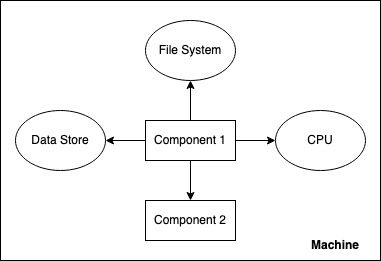
It is difficult to horizontally scale such systems because they do not understand “not here” or “multiple”. Additionally, their implementation might assume that reaching out to these other components is cheap/fast. In distributed systems, both aspects are critical. A subcomponent doing a part of the computations may be running on some other server entirely and therefore difficult to find and expensive to communicate with. A database may be many servers working as a sharded cluster.

Location coupling is therefore a key problem in being able to horizontal scalability because it directly prevents resources from being added “elsewhere”.

Breaking Location coupling

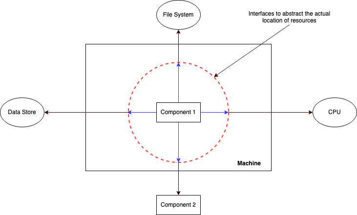
The trick to breaking location coupling lies in abstracting the specifics of accessing another part of the system (file system, database, subcomponent) from the part which wants to access it behind an interface. This means different things in different scenarios.

e.g. at the network layer, we can use DNS to mask the specific IP addresses of remote servers. Load balancing techniques can hide that there are multiple instances of some particular system are running to service high workloads. Smart clients can hide the details of database/cache clusters.

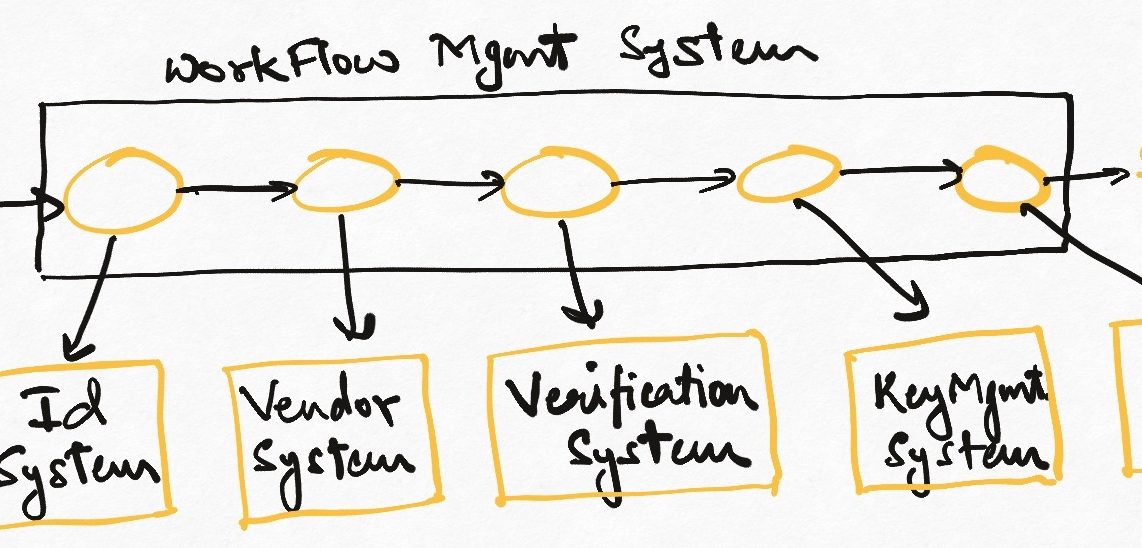
An interesting way of becoming agnostic to the called system physical location is by not trying to locate them but by leaving all commands in a common, well-known place (like a message broker) from where they can up the commands and execute them. This, of course, creates location coupling with the well-known location but ideally, this is smaller in magnitude than having all parts of the system being coupled to all others.

Temporal Coupling

This is the situation where a part of a system expects all other parts on which it depends to serve its needs instantaneously (synchronously) when invoked.

In the context of scalability, the problem with temporal coupling is that all parts must now be “scaled up” at the same time because if one fails, all its dependent systems will also fail. This makes the overall architecture sensitive to local spikes in workload – any change in load on any part of the system and the whole system can crash, thereby removing much of the benefits of horizontal scaling.

Breaking temporal coupling

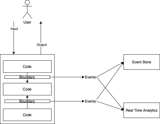
The most common approach to breaking temporal coupling is the use of message queues. Instead of invoking other parts of a system “synchronously” (invoking and waiting till the output appears), the calling system puts a request on a message bus and the other system consumes this

You can read more about messaging concepts and how events can be used to build evolutionary architectures. The event/message-driven architecture can massively increase both the scalability and resilience of a distributed system.